Intro to AI - Udacity
Unit 1 - Intro
Intelligent Agents
- An AI program is called an Intelligent Agent
- Intelligent agents perceive the environment with its sensors and affect the environment’s state with its actuators. The big question of AI is finding the function that maps sensors to actuators. This is also known as a control policy for the agent.
- The process of the agent perceiving through its sensors, deciding what to do, then interacting with the environment with its actuators is called the perception-action cycle. The agent goes through this cycle several times.
Terminology
- An environment is fully observable if only whatever your agent can sense at a given time is sufficient to make the optimal decision.
- An environment is partially observable if the agent requires memory to make the optimal decision.
- A deterministic environment is one where your agent’s actions uniquely determine the outcome.
- A stochastic environment is one where your agent’s actions cannot uniquely determine the outcome, as there is some sort of randomness involved.
- A discrete environment is one where the agent has a finite number of action choices and a finite number of things you can sense.
- A continuous environment is one where the space of possible actions or things you can sense may be infinite.
- A benign environments, the environment might be random, stochastic, but it has no objective of its own that would contradict your objective.
- An adversarial environment, the environment might be random, stochastic, but it has an objective of its own to contradict your objective.
Unit 2 - Problem Solving
Definition of a Problem
- Parts of a problem
- The initial state the agent starts with
- A function, actions, that takes a state as input, and returns a set of possible actions for the agent when in that state.
- A function, result which takes a state and an action as input, and returns a new state.
- A function, goaltest, which takes a state as input and returns a true or false depending on whether the input is a goal or not.
- A function, pathcost, which takes a path(a sequence of state action transitions) and returns the cost of that path.
- A stepcost function takes a state, an action, and the resulting state from that action and returns the cost of that action.
Tree Search Algorithm
function tree_search(problem):
  fringe = {Initial}
  loop:
    if fringe is empty : return FAIL
    path = remove_choice(fringe)
    s = path.end
    if s is a goal : return path
    for a in actions:
      add [path + a -> result(s,a)] to fringe
- Starts by initializing the fringe to be a path only holding the initial state. Then enters a loops where it first checks to see if there is anything left in the fringe. If there is nothing left, the program fails. If there is something left in the fringe, we choose a path and remove it from the fringe. Then we set s to be the last state of the chosen path. Then if that final state is a goal, we return the path. If that final state is not the goal, then we expand that path. We look at all the actions that can be done at that state, and append the old path, the action, and the result of that action to the fringe.
Graph Search Algorithm
function graph_search(problem):
  fringe = {Initial}; explored = {}
  loop:
    if fringe is empty : return FAIL
    path = remove_choice(fringe)
    s = path.end; add s to explored
    if s is a goal : return path
    for a in actions:
      add [path + a -> result(s,a)] to fringe
      unless result(s,a) is in fringe and explored
- This algorithm is similar to the tree search algorithm, but with a few added steps. When we start the search, we initialize the explored set which holds the states that we have already explored. Then when we choose a new path, we add it to the set of explored states. Also, when we expand the new path, we don’t add in a state if we have already encountered that state in the fringe or the explored sets.
Search Algorithms
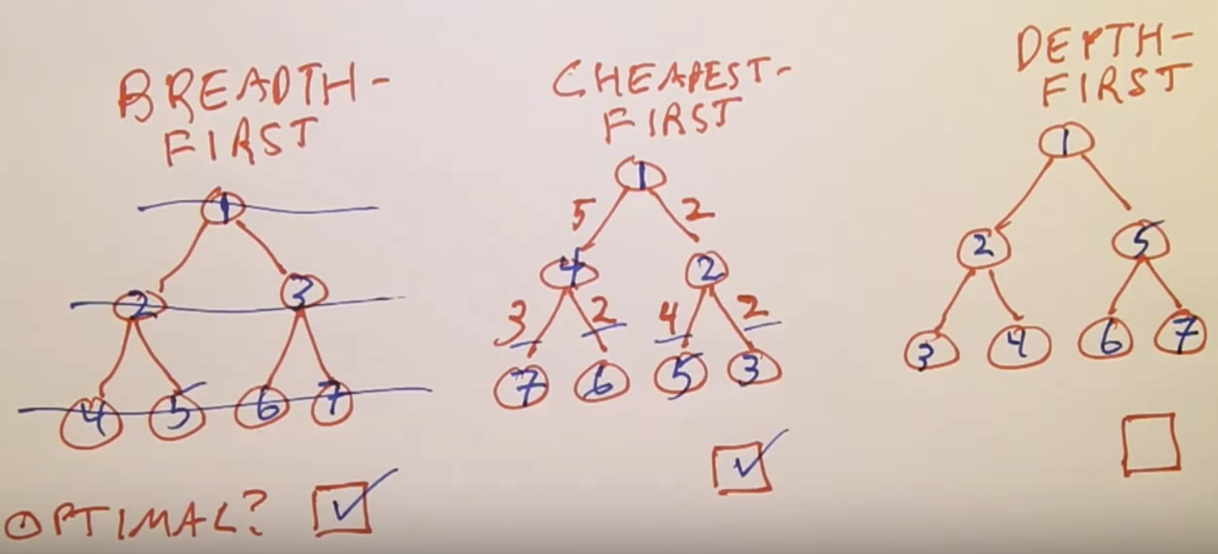
Breadth First Search
- This search algorithm always chooses the shortest possible path off the fringe.
- This algorithm is complete.
Uniform Cost Search(Cheapest First Search)
- This search algorithm always chooses the path with the path with the lowest total cost off the fringe.
- This algorithm is complete.
Depth First Search
- This search algorithm always chooses the longest possible path off the fringe.
- This algorithm is not complete.
Greedy Best First Search
- This algorithm always chooses the path with the least distance to the goal. It expands nodes that get continuously closer to the goal node.
- This algorithm does not always return the shortest path if there are obstacles in the way.
A* Search
- This algorithm always expands the with the minimum value of the function f. The function f is the sum of the path cost and the heuristic of the final state in the path.
- This algorithm finds the lowest cost path if the h(heuristic) cost for a state is less than the true cost of the path to the goal through that state. Another way to state this condition is that h is optimistic, or admissible. An admissible heuristic also never over estimates.
State Spaces
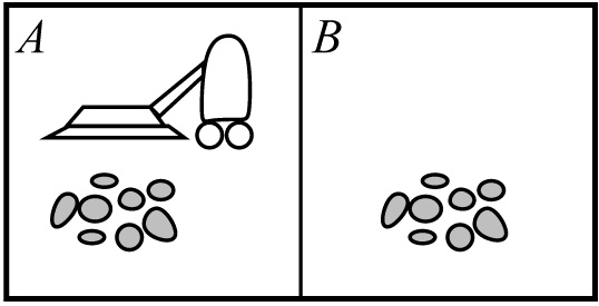
- An example of a state space is the vacuum world shown below. In this space, the vacuum can be in either space a or b. Also, space a or b can be dirty or clean.
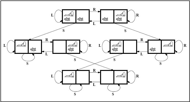
- The state space above has 8 spaces because there are 2 places where the vacuum can be, and 4 combinations of the spaces to be dirty and clean. The diagram of all the states in the state space are shown below.
Constraints of Problem Solving Technology
- Problem solving technology only works when:
- the domain is fully observable(must be able to see the initial state)
- the domain is known(all the possible actions must be known)
- the domain is discrete(must be a finite number of actions to choose from)
- the domain is deterministic(result of taking an action must be known)
- the domain is static(nothing else in the world that can change the world except for our own actions)
Implementation of Search Algorithms
- With search algorithms, we talk a lot about paths in the state space. When implementing paths in computer programs, we make use of nodes. A node is a data structure with the four fields.
- The fields of a node are
- state - State at the end of the path
- action - The action the algorithm took to get to the state
- cost - Total cost of the path
- parent - A pointer to another node before it.
- The two data structures that utilizes nodes in search algorithms are the fringe and the explored set
- Since we add and remove nodes from the fringe, which means it should be implemented as a priority queue. However, there must also be a check to see if a node is in the fringe, so it can also be implemented as a hashmap or a tree.
- With the explored set, we just add new nodes and check if nodes are in the set. So this can be implemented with hashmap or a tree as well.
Unit 3 - Probability in AI
Bayes Network
-
A Bayes Network is a compact representation of a distribution over this very large joint probability distribution or all the variables.
-
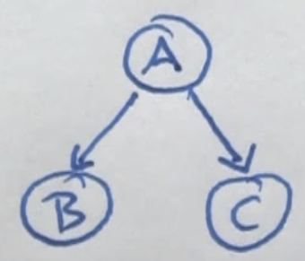
A Bayes Network is composed of nodes and these nodes correspond to events that you may or may not know(random variables). These nodes are connected with arcs and an arc suggests that the child of the arc is influenced by the parent. It may not be influenced in a deterministic way, but may be influenced in a probabilistic way.
Probabilities
- Complimentary probability - \(P(A) = p \to P(\bar{A}) = 1-p\)
- Independence - If two variables, x and y, are independent, then the joint probability of the two variables is the product of probability of x and probability or y.
- Law of Total Probability - \(P(Y) = \sum_{i} P(Y|X=i) \cdot P(X=i)\)
- Negation of probabilities - \(P(\bar{X}|Y) = 1 - P(X|Y)\)
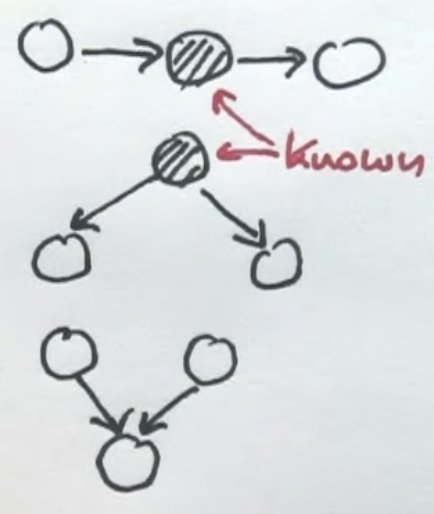
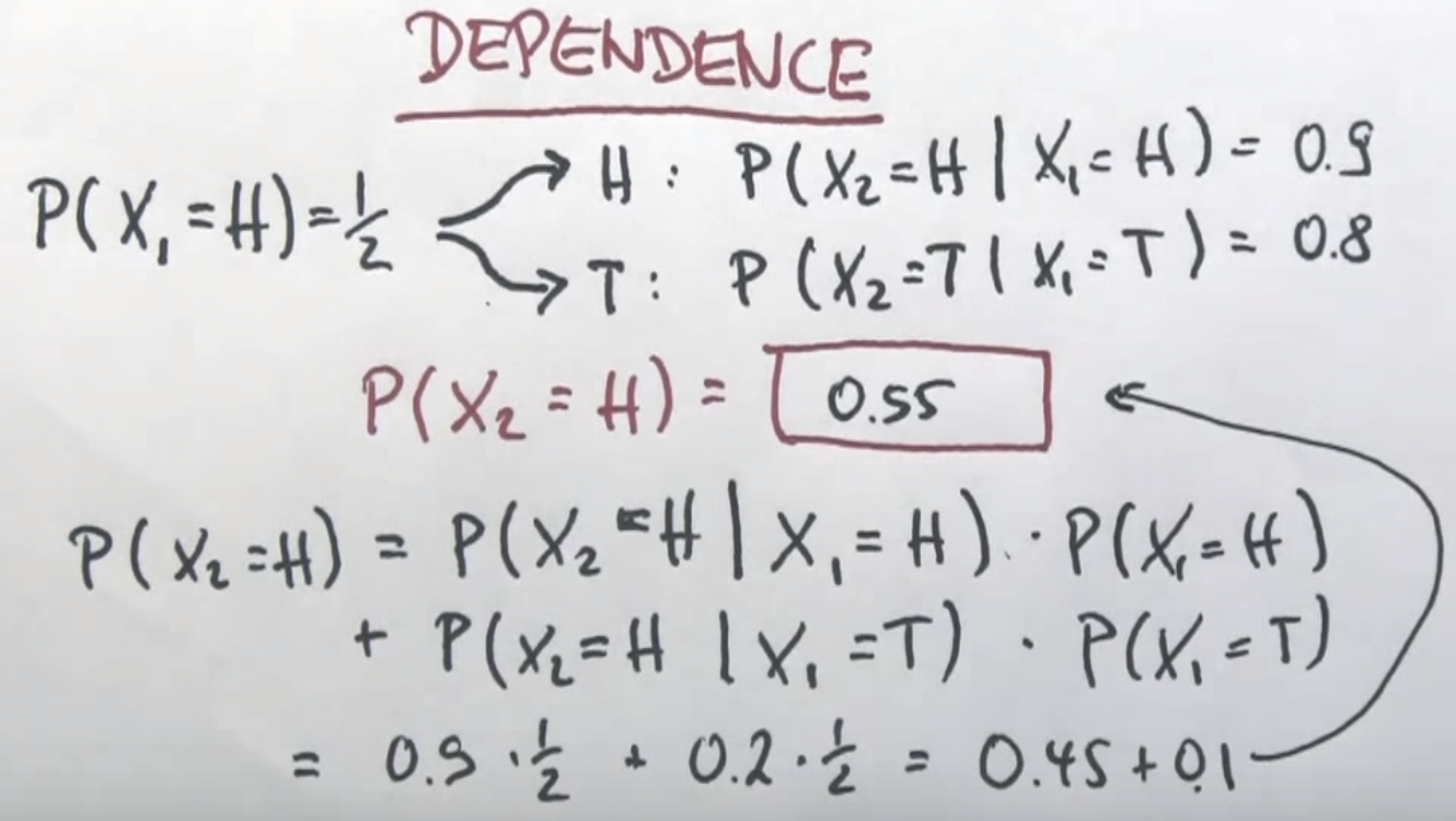
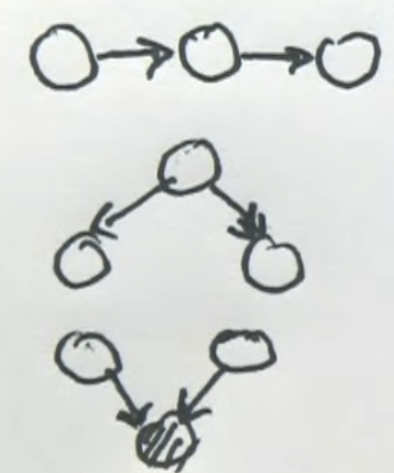
- Dependence - One probability depends on the probability of another event. An example of a dependence problem is shown below.
- Conditional Independence - Given the Bayes Network shown below, if given A, then B is independent of C.
- Conditional independence does not imply absolute independence and absolute independence does not imply conditional independence.
Bayes Rule
-
Bayes Rule - \(P(A|B) = \frac{P(B|A) \cdot P(A)}{P(B)}\) or \(P(\bar{A}|B) = \frac{P(B|\bar{A}) \cdot P(A)}{P(B)}\)
-
We can write Bayes rule differently by just writing it with ignoring the normalizing terms(denominators). This gives us the equations below.
- Then, we must get the original probability by normalizing the equations. We do this by using the equation above and the traditional definition of Bayes rule, we get the following equations
- The factor \(\eta\) is the normalizing factor. The equation for \(\eta\) is given below.
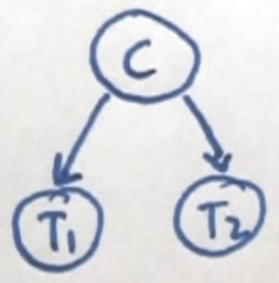
Two Test Cancer Example
Terminology
- Probability of positive cancer test = \(P(+)\)
- Probability of negative cancer test = \(P(-)\)
- Probability of having cancer = P(\(C\))
- Probability of not having cancer = P(\(\bar{C}\))
Given info:
| \(P(C) = 0.01\) | \(P(\bar{C}) = 0.99\) |
| \(P(+|C) = 0.9\) | \(P(-|C) = 0.1\) |
| \(P(-|\bar{C}) = 0.8\) | \(P(+|\bar{C}) = 0.2\) |
Problem:
Find \(P(C|++)\).
To find \(P(C|++)\) we can utilize Bayes rule.
| \(P(C)\) | \(+\) | \(+\) | \(P'\) | |
| \(C\) | 0.01 | 0.9 | 0.9 | 0.0081 |
| \(\bar{C}\) | 0.99 | 0.2 | 0.2 | 0.0396 |
Then by adding the \(P'\) probabilities and then inverting, we calculate \(\eta\) is 20.9644. Then by multiplying the \(\eta\) factor by the \(P'\) values, we can calculate that \(P(C|++) = 0.1698\).
Problem:
Find \(P(T_{2}=+|T_{1}=+)\).
To find \(P(T_{2}=+|T_{1}=+)\) we can utilize the Theorem of Total Probability. With that, we can write the following equation.
\[P(T_{2}=+|T_{1}=+) = P(T_{2} = +|T_{1} = +, C) \cdot P(C|T_{1} = +) + P(T_{2} = +|T_{1} = +,\bar{C}) \cdot P(\bar{C}|T_{1} = +)\]Then by evaluating the expression, we get that \(P(T_{2}=+|T_{1}=+) = 0.2301\).
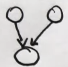
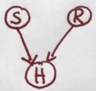
Confounding Cause Bayes Networks
-
Confounding cause Bayes networks are like the traditional Bayes networks that we studied before, just with two independent hidden causes that get confounded into a single observational variable.
-
The general shape of a Bayes network for confounding cause is shown below.
Happiness Example
Terminology
- Probability of being sunny = \(P(S)\)
- Probability of raise = \(P(R)\)
- Probability of happiness = P(\(H\))
- Probability of not happiness = P(\(\bar{H}\))
Given info:
| \(P(S) = 0.7\) |
| \(P(R) = 0.01\) |
| \(P(H|S,R) = 1\) |
| \(P(H|\bar{S},R) = 0.9\) |
| \(P(H|S,\bar{R}) = 0.7\) |
| \(P(H|\bar{S},\bar{R}) = 0.1\) |
Problem:
Find \(P(R|S)\).
We can immediately say that \(P(R|S) = 0.01\) because the information of a sunny day(S) or getting a raise(R) affect happiness, but they don’t affect each other. This means that they are independent of each other.
Problem:
Find \(P(R|H,S)\).
We can expand \(P(R|H,S)\) by utilizing Bayes rule. The resulting equation is given below.
\[P(R|H,S) = \frac{P(H|R,S) \cdot P(R|S)}{P(H|S)}\]Then by observing the conditional independence of R and S, we can simply the equation to
\[\frac{P(H|R,S) \cdot P(R|S)}{P(H|S)} = \frac{P(H|R,S) \cdot P(R)}{P(H|R,S) \cdot P(R) + P(H|\bar{R},S) \cdot P(\bar{R})}\]The by utilizing the given information, we can state that \(P(R|H,S) = 0.0142\).
Problem:
Find \(P(R|H)\).
We first find the variable \(P(H)\). The value of the variable is shown below.
\[P(H) = P(H|S,R) \cdot P(S,R) + P(H|\bar{S},R) \cdot P(\bar{S},R) + P(H|S,\bar{R}) \cdot P(S,\bar{R}) + P(H|\bar{S},\bar{R}) \cdot P(\bar{S},\bar{R})\]This can be expanded by plugging in the values from the given data above.
\[P(H) = 0.5245\]Then by using Bayes rule, we can get an equation for \(P(R|H)\).
\[P(R|H) = \frac{P(H|R) \cdot P(R)}{P(H)}\]We know the value of \(P(R)\) from the given information and we can get an equation for \(P(H|R)\) using the Law of Total Probability.
\[P(H|R) = P(H|R,S) \cdot P(S) + P(H|R,\bar{S}) \cdot P(\bar{S}) = 0.97\]So now that we have all the values we need, we can plug them into the equation for \(P(R|H)\).
\[P(R|H) = \frac{0.97 \cdot 0.01}{0.5245} = 0.0185\]Conditional Dependence
- In the examples using the Bayes network about happiness, we see that if the problem doesn’t reference anything about happiness, then the probability of getting a raise the probability for it being sunny are independent. However, when we introduce information about happiness, it introduces a dependence on R and S. This is known as conditional dependence.
General Bayes Networks
-
Bayes Networks define probability distributions over graphs or random variables.
-
We can find the number of probability values needed to specify a specific bayes network by summing the amount of values needed per node. We can calculate the number of probability values needed at each node by using the equation \(Values = 2^{N}\), where N is the number of incoming arcs at the particular node.
D-Separation
-
Any 2 variables are independent if they’re linked with nodes that we know the value of.
- Active triplets
- Render them dependent
- Some examples of active triples are
- Inactive triplets
- Render them independent
- Some examples of inactive triples are