Microeconomics
Microeconomics
Syllabus
- Opportunity cost - The cost of choosing a specific opportunity and also the cost/value of the opportunities that you did not take.
- Marginal - means “additional”
- An example of this is
Scenario 1
---------
A summer course runs for the whole summer. The course fees are $1,300.
If you don't take the course, you could work at Job A which pays $7000 OR Job B
which pays $6000. Both courses take the entire summer.

Opportunity cost of taking the course: $8,300 (course fee + highest forgone
alternative) -> Took the course and forgo the Jobs money(only Job A because
it is the highest and you could only choose one Job out of the two)

Scenario 2
---------
A summer course runs for the whole summer. The course fees are $1,300.
If you don't take the course, you could work at Job A which pays $7000 AND Job B
which pays $6000. Job A takes the first half of the summer, and Job B takes the
second.

Opportunity cost or taking the course: $14,300 (course fee + highest forgone
alternatives) -> Took the course and forgo the Jobs money

Scenario 3
---------
A summer course runs for half the summer. The course fees are $1,300.
If you don't take the course, you could work at Job A which pays $7000 OR Job B which pays $6000. Both courses take the entire summer.

Opportunity cost of taking the course: $8,300 (course fee + highest forgone alternative) -> Took the course and forgo the Jobs money(only Job A because it is the highest and you could only choose one Job out of the two)

Scenario 4
---------
A summer course runs for half the summer. The course fees are $1,300.
If you don't take the course, you could work at Job A which pays $7000 AND Job B which pays $6000. Job A takes the first half of the summer, and Job B takes the second.

Opportunity cost or taking the course: $8,300 (course fee + highest forgone alternatives) -> Took the course and forgo the money from Job A
Chapter 3 : Optimization : Doing the best you can
- Optimal Choice - “X is the best(optimal)” choice
Exercise 1
----------
(Optimization in Levels) Suppose that there are 3 possible airports near your
home that you use for a flight to Boston. At the closest airport you find an
airfare of $400, the middle airport has an airfare of $325, and you would pay
$275 to fly from the furthest airport. Assume you want to take the taxi to the
airport and the round trip cost to the close airport is $20 and will take 15
minutes. The taxi fare to the second airport is $30 and will take 30 minutes.
The taxi fare to the furthest airport is $60 and will take one hour. You have a
 part-time job where you earn $12 per hour. Create a table and determine which
 airport is the optimum for you to use.
| Airport | Time to Airport | Cost of Travelling to Airport | Taxi Fare | Airfare | Total Cost |
|---|---|---|---|---|---|
| Closest | 15 min | 3 | 20 | 400 | 423 |
| Middle | 30 min | 6 | 30 | 325 | 361 |
| Furthest | 60 min | 12 | 60 | 275 | 347 (Optimal) |
Exercise 2
----------
(Optimization in Levels : Comparative Statistics) Use all the data from exercise
 1 for this problem. Assume you have a next door neighbor who is a lawyer who
 earns $200 per hour. Create a table and determine which airport is the optimum
 for your neighbor to use.
| Airport | Time to Airport | Cost of Travelling to Airport | Taxi Fare | Airfare | Total Cost |
|---|---|---|---|---|---|
| Closest | 15 min | 50 | 20 | 400 | 470 |
| Middle | 30 min | 100 | 30 | 325 | 455 (Optimal) |
| Furthest | 60 min | 200 | 60 | 275 | 535 |
Exercise 3
----------
(Optimization in Differences : Marginal Analysis) Use the data from exercise 1
for this problem. Create a table using marginal cost analysis to confirm that
the answer for exercise 1 is the same when marginal analysis is used confirm the
answer for exercise 1 is the same when marginal analysis is used instead of
optimization in levels.
| Airport | Time to Airport | Cost of Travelling to Airport | Taxi Fare | Airfare | Total Cost | Marginal Cost |
|---|---|---|---|---|---|---|
| Closest | 15 min | 3 | 20 | 400 | 470 | |
| Middle | 30 min | 6 | 30 | 325 | 455 | -62(from closest) |
| Furthest | 60 min | 12 | 60 | 275 | 535 | -14(from middle) (OPTIMAL) |
- Marginal Analysis is analyzing the difference between two options in the table
Challenge for Problem 3
---------------------
If the value of time is less than or equal $X per hour, then FURTHEST is the
optimal choice.
"What is the least cost of time so that the furthest airport to be the
optimal choice, using the values given in exercise 3?"

Answer = $40
| Airport | Time to Airport | Cost of Travelling to Airport | Taxi Fare | Airfare | Total Cost |
|---|---|---|---|---|---|
| Closest | 15 min | X/4 | 20 | 400 | 420 + (X/4) |
| Middle | 30 min | X/2 | 30 | 325 | 355 + (X/2) |
| Furthest | 60 min | X | 60 | 275 | 335 + X |
- We use the derived total costs for each airport and then calculate the Marginal Cost for each airport compared to the Furthest. To compare them we would put them in the equation (Airport A Total Cost) <= (Total Cost of Airport B).
Difference between Opportunity Cost and TOTAL Opportunity Cost
-
You have $1,000 to by a guitar. Instead of buying the guitar, you can invest in stock. This will earn 5% on investment -> $50. What is the total opportunity cost and the opportunity cost of buying the guitar?
- Total Opportunity Cost = $1,050(includes the $1,000 investment and the amount of money lost by not choosing the other option)
- The Opportunity Cost = $50(the cost difference of no choosing the other option compared to the option you chose)
Some examples of Optimal choice
**Example 1**
1. Trade-offs and Opportunity Cost
You spend your time between surfing the web and working. Surfing the web pays
nothing(but you get some pleasure) while the hourly wage from working is $8.40.
When you have money, you spend it on music: each song you download costs $1.20.
Obviously, the more time you spend surfing the web, the fewer songs you can
afford. What is the marginal cost(also known as the opportunity cost), measured
by the number of songs you have to give up, if spending one more hour
on surfing the web? Explain your answer.
Answer
- Surfing the web for 1 hour is, essentially, losing $8.40.
- In terms of songs, each song is $1.20, so surfing the web for 1 hour is losing 7 songs
**Example 2**
2. Optimization in Difference(Marginal Analysis)
The table below shows the commuting time and the apartment rent at four
locations you are considering to live.

(a) If the monthly rent at the Close location is $1,900 and if you value your
time at $40/hour, is it worth choosing Close over Very Close? What location is
optimal for you? Be sure to apply optimization in difference.

(b) Suppose that you value your time at $60/hour and you optimal choice is
Close. Then the monthly rent at Close must be at most $_____. Explain your
answer.
| Location | Commuting Time / mo. | Rent / mo. |
|---|---|---|
| Very close | 4 hours | $2,200 |
| Close | 11 hours | ??? |
| Far | 20 hours | $1,400 |
| Very Far | 32 hours | $1,000 |
Answer
- (a)
- Close = (11 hours) * ($40/hour) + $1,900
- Very Close = (4 hours) * ($40/hour) + $2,200
- Close is the optimal choice
- (b)
- Close = (11 hours) * ($60/hour) + X = $660 + X
- Very Close = (4 hours) * ($60/hour) + $2,200 = $2,440
- ($660+X) </= $2,440, which makes X </= $1,780
Chapter 4: Demand, Supply, Equilibrium
- Demand
- You (the consumer) have a demand for a good or service if …
- you can afford it
- Depends on price of the object and your budget
- you plan to buy it
- Depends on prices of other related goods
- Depends on preferences/taste
- you can afford it
- You (the consumer) have a demand for a good or service if …
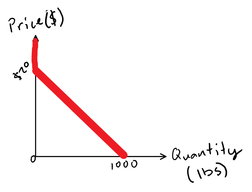
- Demand Curve - A curve which shows the relationship between the price of a good and the quantity demanded.
- When you draw a demand curve, measure price on the vertical axis
-
- If income, prices of other related goods and/or your preferences change, you have to draw a new demand curve
- An example of a demand curve is
When Does a Demand curve shift rightward?
- If the income of the consumer goes up, then the demand curve would shift right
- Consumers Income(budget) increases
- Price of a substitute increases
- Price of a compliment decreases
- Positive information about the good
- Changes in consumer’s taste for the good
- Expectation that the price of the good will go up in the future.
-
The Law of Demand - If the price of the product goes up, the quantity demand goes down
-
A perfectly competitive market is fiction
-
Equilibrium Price - The price where the quantity demanded equals the quantity supplied
- Supply Curve - A curve which shows the relationship between the price of a good and the quantity supplied.
**Example of shifting the demand curve**
The Super Bowl in 2014 was held outdoors in New Jersey in the winter. Assume the
market for tickets to the event was in equilibrium one week prior to the Super
Bowl. A weather report forecasted cold weather for the event, and the price for
outdoor seats fell. On one website, the prices fell from $2,233 to $1,395 per
ticket. The price for club seats that included access to a heated area did not
change during the week before the event. Show the effect of the weather report
in a graph.
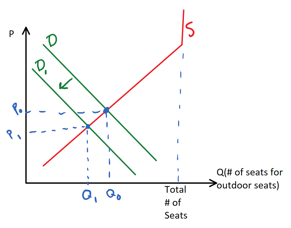
- The portion of the supply curve that is vertical represents the time when no more tickets can be supplied no matter how high the price is
- The demand curve will shift to the left as the demand decreases due to the predicted weather conditions
- The point \(\( Q_0, P_0 \)\) represents the equilibrium point before the weather report
- \[P_0 = $2,233\]
- The point \(\( Q_1, P_1 \)\) represents the equilibrium point after the weather report
- \[P_0 = $1,395\]
How to “look at(interpret)” a demand curve
- Demand Curve tells us the quantity demanded at each price
- Example Interpretation: “The customer is willing to pay at most $1.50 for 100 units”
- For each (additional) unit, the demand curve tells us the maximum amount of money the customer is willing to pay for it
- Example Interpretation: “For the 100th unit, the customer is willing to pay at most $1.50”
How to “look at(interpret)” a supply curve
- A supply curve tells us the quantity supplied at each price
- Example Interpretation: “At the price of $1.50, the seller(s) is willing to sell 100 units”
- A supply curve tells us the minimum acceptable price for the seller to sell each (additional) unit
- Example Interpretation: “Seller is willing to sell the 100th unit for at least $1.50”
- Where does minimum acceptable cost come from?
- It’s the cost of making that unit - It’s the same as the marginal cost