Intro to AI
Introduction
What is Intelligence?
- According to the Oxford dictionary, intelligence is the ability to acquire and apply knowledge and skills.
- Intelligence is a goal-directed adaptive behavior
What is AI?
- There have been 4 approaches to AI that have been followed in history
- Thinking Humanly
- Acting Humanly
- Thinking Rationally
- Acting Rationally
Thinking Humanly
- For a program to think like a human, we must know how we think. We use introspection to observe our thoughts. We use psychological experiments to observe a person’s actions and we use brain imaging to observe the brain during all of this.
Acting Humanly
- The Turing test - used to provide an operational definition of intelligence.
- A human interrogator is placed in a room, with a computer placed in the room next door. The interrogator then poses questions to the room and the computer passes the test if the human cannot tell whether the response comes from a human or a computer.
- To pass the Turing test, the computer needs to posses the following:
- Natural Language Processing
- Knowledge Representation
- Automated Reasoning
- Machine Learning
- For the complete Turing test, the program would also posses computer vision to interpret the question, and robotics to manipulate objects to write a response.
Thinking Rationally
- Rationality: being reasonable, based on facts or reason; doing the right thing.
- Aristotle, a Greek philosopher, was one of the first to attempt tot codify rational thinking. He created syllogisms to provide patterns that always yielded correct conclusions when given the correct inputs.
Acting Rationally
- AI is the discipline of studying and designing rational agents.
Agents
- An agent is something that can perceive its environment through sensors and acting upon that environment through actuators.
- Precept - the agent’s perceptual inputs at any given instance. A precept sequence is the complete history of what the agent has perceived.
- The agent function maps any given precept or precept sequence to an action.
- A rational agent is an agent that acts to achieve the best expected outcome.
- To measure the performance of an agent, we must define a measure of performance. Some way to quantize the performance of the agent.
- Properties of agent environments are defined in the table below.
| Fully Observable | Only whatever your agent can sense at a given time is sufficient to make the optimal decision |
| Partially Observable | The agent requires memory to make the optimal decision |
| Deterministic | An environment where your agent’s actions uniquely determine the outcome. |
| Stochastic | An environment is one where your agent’s actions cannot uniquely determine the outcome, as there is some sort of randomness involved. |
| Discrete | An environment is one where the agent has a finite number of action choices and a finite number of things you can sense. |
| Continuous | An environment where the space of possible actions or things you can sense may be infinite. |
| Benign | The environment might be random, stochastic, but it has no objective of its own that would contradict your objective |
| Adversarial | The environment might be random, stochastic, but it has an objective of its own to contradict your objective. |
| Single Agent | The environment only contains one agent at a time. |
| Multiagent | The environment may contain several agents at a time. |
| Episodic | An environment where an agent only has to do one action to complete its task. |
| Sequential | An environment where an agent must take more than one action to complete its task. |
| Known | An environment where the agent knows all the possible attributes of the environment. |
| Unknown | An environment where the agent doesn’t know the attributes of the environment. |
IN THIS COURSE, WE ASSUME THAT THE ENVIRONMENT IS KNOWN AND FULLY OBSERVABLE, AND ACTIONS ARE DETERMINISTIC. THE ENVIRONEMENTS WILL ALSO BE SINGLE AGENT.
Solving Problems by Searching
- A well defined problem is described by
- States - set of all possible situations
- Initial state - starting state
- Goal state(s) - destinations or final positions
- Goal test - determines whether a given state is a goal state
- Actions - set of everything an agent can do to change its current state.
- Transition model - the effect of each action
- Path cost - function that assigns a numeric cost to each path.
-
The initial state, actions, and transition model together implicitly define the state space of a problem.
- A path is a sequence of states connected by a sequence of actions.
- The cost of a path is the sum of the costs of the individual actions along the path. The step cost of an action, \(a\), in state \(s\) to reach state \(s'\) is denoted by \(c(s,a,s')\).
- A solution to a problem is a sequence of actions that leads from the initial state to the goal state. A solution with the lowest path cost is an optimal solution.
Vacuum World Example
This world contains a vacuum the two rooms, A and B. The vacuum has the actions left/right to move between rooms, and suck to get rid of the dirt in a given room.
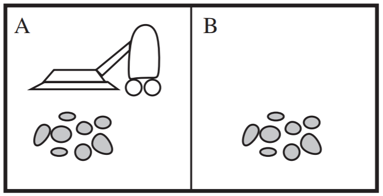
The state space of the problem is shown below.
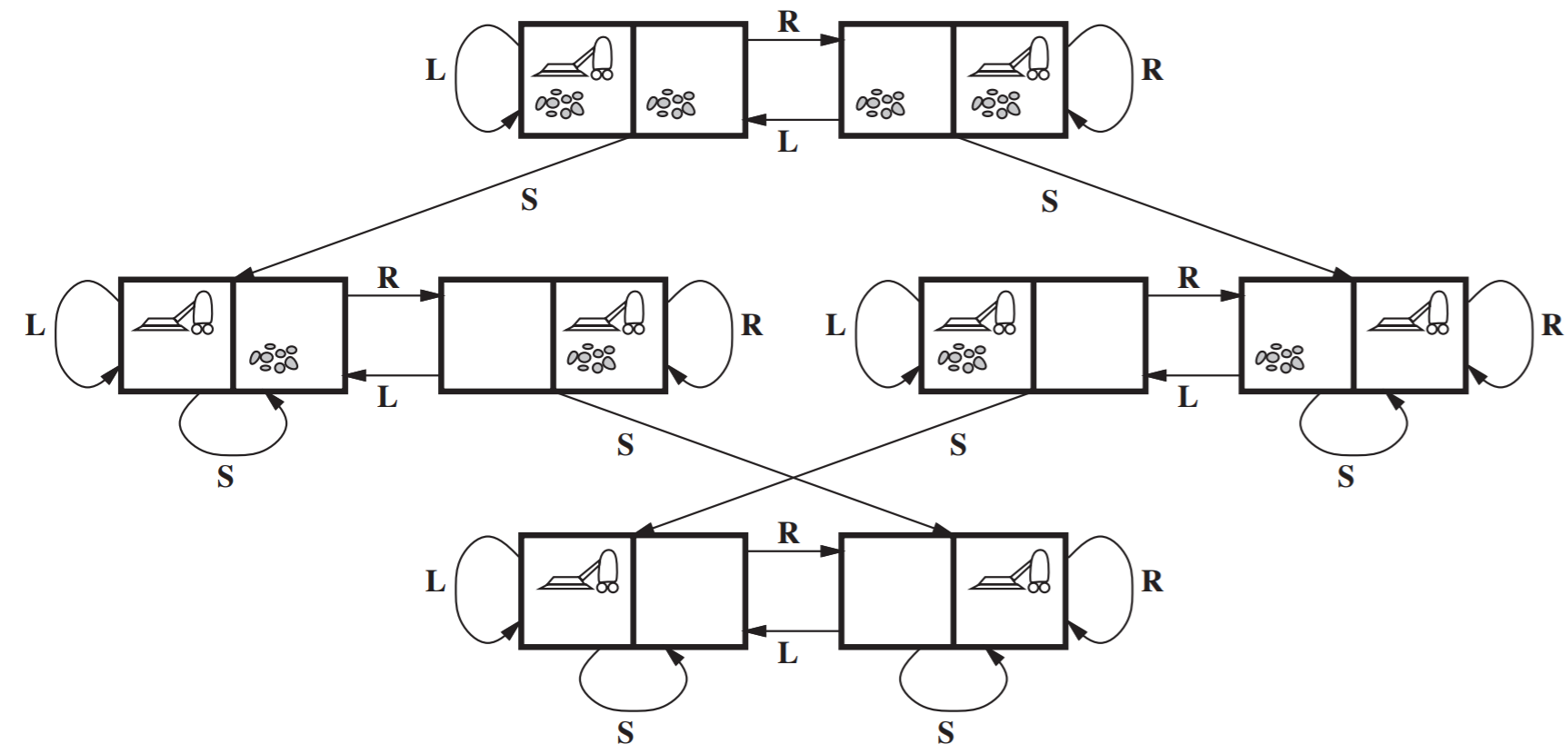
The formal description of the Vacuum World is
- States: There are 2 rooms that may or may not contain dirt and there are 2 positions for the robot. There are \(2 \cdot 2^{2} = 8\) possible world states.
- Initial State: Any state can be the initial state.
- Goal State: Having both the rooms clean. This is seen in the bottom two states of the state space.
- Actions: Move left, Move right, suck
- Transition model: The actions have their expected effects. Moving left or right, moves the robot accordingly. Moving left in the left space or moving right in the right space have no effect on the position of the robot.
- Path cost: Each action has a cost of 1.
Search Trees
- A solution to a problem is an action sequence. Search algorithms work by considering various possible action sequences and finding the optimal one as a solution. All the possible action sequences starting from the initial state from a search tree with the initial state at the root. The branches are actions and the nodes correspond to the states in the problem’s state space.
- The process of finding the goal state in the tree is called tree searching
Tree Search
- A node is expanded when all it’s children are added to the search tree.
- The set of nodes that have already been added to the search, but have not yet been expanded is called the open list, fringe, or frontier.
- A generic algorithm for tree searching is
function tree_search(problem):
  fringe = {Initial State}
  loop:
    if fringe is empty : return FAIL
    s = remove_choice(fringe)
    if s is a goal : return path taken to goal
    for a in actions: //Expand current node
      add [result(s,a)] to fringe
- The tree search starts by initializing the fringe with the initial state of the problem. Then enters a loop where it first checks to see if there are any nodes in the fringe. If there are no nodes, it returns a failure. If there are nodes in the fringe, we choose a node, s, and remove it from the fringe. If s is a goal state, the program then returns the path it took from the root to node s. If it is not a goal state, then we expand state s. We look at all the actions that can be done at the state, and add the resulting nodes to the fringe.
- Search algorithms vary with the way they remove from and add to the fringe. They only vary in the function
remove_choice()from the algorithm above.
Implementing a Search Tree algorithm
- In a search tree, each node, n, is represented by a data structure that contains the fields of
- n.State: the state the node corresponds to
- n.Parent: the parent of node n
- n.Action: the action from n.Parent that leads to node n
- n.Path-cost: the cost of the path from root to the current node, denoted by \(g(n)\)
- n.Depth: number of nodes from root to current node including the current node
- A generic child node is
function CHILD-NODE(problem, parent, action) returns a node
  return a node with
    STATE = problem.RESULT(parent.STATE, action),
    PARENT = parent, ACTION = action,
    PATH-COST = parent.PATH-COST + problem.STEP-COST(parent.STATE, action)
- The nodes are kept in a queue. The operations on a queue are
- EMPTY?(queue): returns true if the queue is empty
- POP(queue): removes the first element and returns it
- INSERT(element, queue): insert an element and returns the resulting queue. This is also known as PUSH().
- INITIALIZE(element): returns a queue that contains the element
- Queues are categorized by the order in which they store the inserted nodes
- FIFO: first-in, first-out
- LIFO: last-in, first-out
- Priority: pops the element with the highest priority according to a priority function
- The four criteria used to compare various search tree algorithms are
- Completeness: Is the algorithm guaranteed to find a solution when there is one?
- Optimality: Does the strategy find the optimal or best solution?
- Time Complexity: How much time does it take to find a solution?
- Space Complexity: How much memory is needed to perform the search?
- The following parameters are used to calculate and compare the performance of an algorithm:
- b: the maximum branching factor(number of children per node)
- If the number of children per parent vary, then we would use an effective branching factor
- d: the depth of the shallowest goal state
- m: the maximum length of a path in the tree
- b: the maximum branching factor(number of children per node)
- The search cost or a search algorithm refers to the time complexity. However, it can also include a term for the memory usage, and when it does, it is known as total cost. This combines the search cost and the path cost of the algorithm.
Graph Search
- The set of expanded nodes is called the closed list or explored list.
- In tree searches, there can be several repeated nodes in the search tree. To avoid these redundant paths, graph searching keeps tracks of explored nodes as well.
- A generic algorithm for graph searching is
function graph_search(problem):
  fringe = {Initial}; explored = {}
  loop:
    if fringe is empty : return FAIL
    s = remove_choice(fringe)
    add s to explored
    if s is a goal : return path to goal
    for a in actions:
      add [path + a -> result(s,a)] to fringe
      unless result(s,a) is in fringe and explored
- This algorithm is similar to the tree search algorithm, but with a few added steps. When we start the search, we initialize the explored set which holds the states that we have already explored. Then when we choose a new node, we add it to the set of explored nodes. Also, when we expand the new node, we don’t add in a node if we have already encountered that node in the fringe or the explored sets to eliminate the redundancy.
Uninformed Search Strategies
- An uninformed search algorithm means the strategies have no additional information about the states beyond that provided in the problem definition.
- Some uninformed search algorithms are
- Breadth-first search
- Uniform-cost search
- Depth-first search
- Depth-limited search
- Iterative deepening depth-first search
- Bidirectional search
Breadth-First Search (BFS)
- BFS expands all the nodes in current level first before expanding the nodes at the next level.
- BFS always has the shallowest path to every node in the frontier.
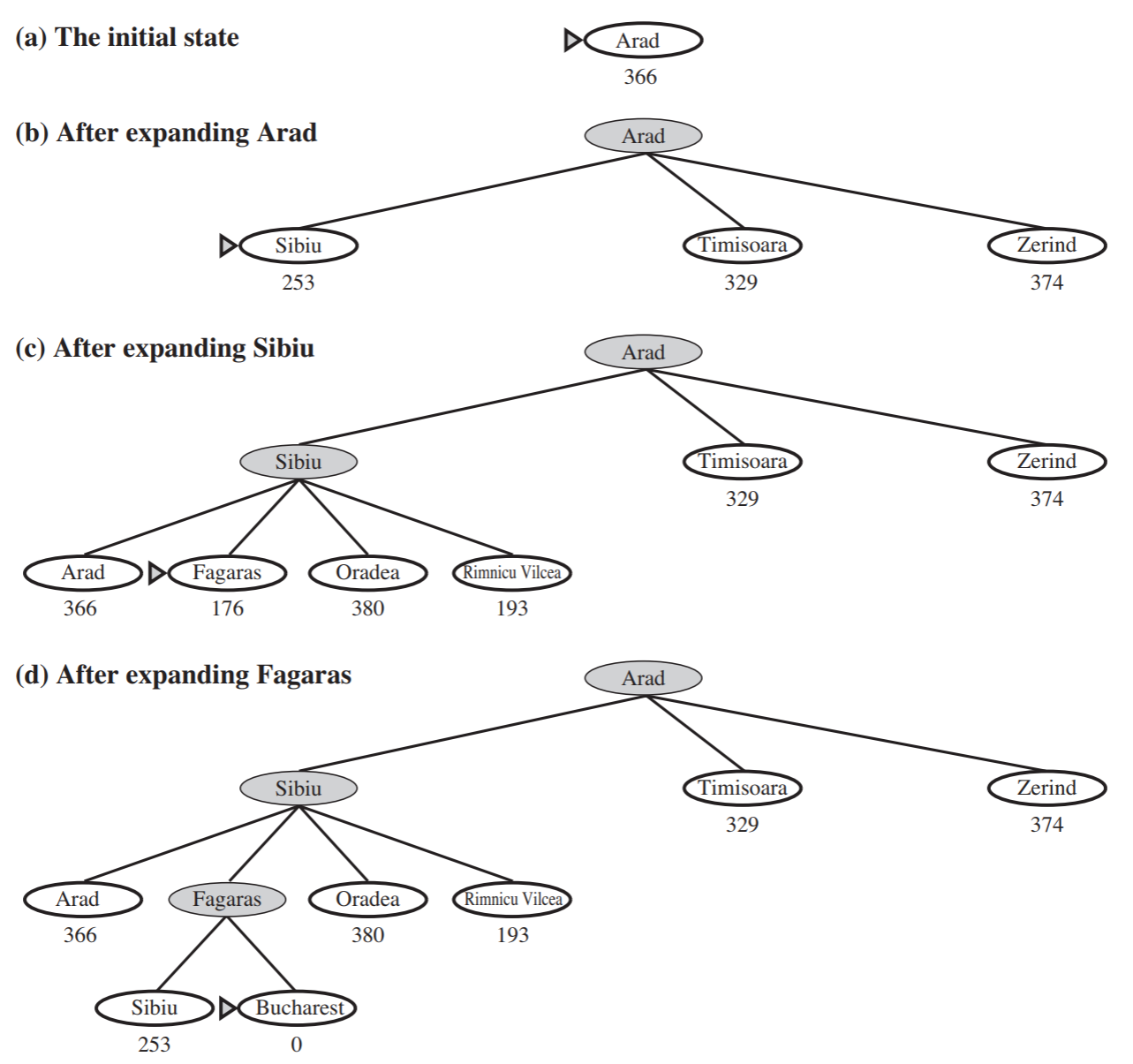
- An example of BFS is
- A generic BFS algorithm is
function BREADTH-FIRST-SEARCH(problem) returns a solution, or failure
  n <- a node with STATE = problem.INITIAL-STATE, PATH-COST = 0
  if problem.GOAL-TEST(n.STATE) then return SOLUTION(n)
  frontier <- a FIFO queue with n as the only element
  explored <- an empty set
  loop:
    if EMPTY?(frontier) then return failure
    n <- POP(frontier) // Chooses the shallowest node in the frontier
    add n.STATE to explored
    for each action in problem.ACTIONS(n.STATE) do
      child <- CHILD-NODE(problem, n, action)
      if child.STATE is not explored or frontier then
        if problem.GOAL-TEST(child.STATE) then return SOLUTION(child)
        frontier <- INSERT(child, frontier)
- The properties of BFS are
- Frontier Queue: First-in First-out (FIFO)
- Completeness: Complete if branching factor, b, is finite
- Optimality: Optimal only if all the costs of the edges are equal(shallowest path in the tree is not always the shortest is the problem)
- Time complexity: \(O(\sum_{i=0}^{d-1} b^i) = O(b^d)\)
- Space complexity: \(O(\sum_{i=0}^{d-1} b^i) = O(b^d)\)
- With an exponential complexity(\(O(b^d)\)) is really inefficient!
Uniform-Cost Search
- BFS is optimal only when all step costs are equal. Uniform-cost search, however, expands the node with the lowest path cost, instead of the shallowest node.
- The queue of the fringe is ordered by path cost.
-
In BFS, all the nodes in the queue have the same path cost, and the goal test is performed when a node is generated. However, in Uniform-cost search, the nodes in the queue have different path costs. The goal test is performed when a node is expanded.
- A generic Uniform Cost Search algorithm is
function UNIFORM-COST-SEARCH(problem) returns a solution, or failure
  n <- a node with STATE = problem.INITIAL-STATE, PATH-COST = 0
  frontier <- a priority queue ordered by PATH-COST, with n as the only element
  explored <- an empty set
  loop:
    if EMPTY?(frontier) then return failure
    n <- POP(frontier) // Chooses the lowest-cost node in the frontier
    if problem.GOAL-TEST(node.STATE) then return SOLUTION(n)
    add n.STATE to explored
    for each action in problem.ACTIONS(node.STATE) do
      child <- CHILD-NODE(problem, node, action)
      if child.STATE is not in explored or frontier then
        frontier <- INSERT(child, frontier)
      else if child.STATE is in frontier with higher PATH-COST then
        replace that frontier node with child
- The properties of Uniform-cost Search are
- Frontier queue: Ordered by path cost
- Completeness: Complete if branching factor is finite
- Optimality: Optimal search
- Whenever uniform-cost search selects a node, n, for expansion, the optimal path node has been found
- Time complexity: \(O(b^{1 +\lfloor C^{*}/\epsilon \rfloor})\), where \(C^*\) is the path cost of the optimal path and \(\epsilon\) is the minimum step cost. There is a factor of 1 before because we start at the root which is position 0, which then contributes the factor of 1.
- Space complexity: \(O(b^{1 +\lfloor C^{*}/\epsilon \rfloor})\), where \(C^*\) is the path cost of the optimal path and \(\epsilon\) is the minimum step cost. There is a factor of 1 before because we start at the root which is position 0, which then contributes the factor of 1.
- Dijksta’s algorithm is a slightly different variant of Uniform-cost search
- Dijksta’s uses a list of unvisited vertices(initially contains all vertices), and a table that keeps track of the shortest distance to each vertex so far(initialized to infinity) instead of open and closed lists.
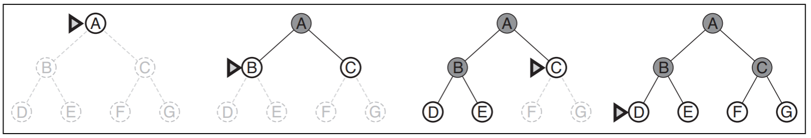
Depth First Search (DFS)
- DFS always expands the deepest node in the frontier first.
- DFS can get stuck in infinite loops if visiting repeated states is allowed, so then it is not complete
- Properties of DFS:
- Frontier queue: Last-in First-out (LIFO)
- Optimality: Not optimal, because it returns the first path that contains the goal.
- Time Complexity: \(O(b^m)\), where m is the maximum depth of any node. This is worse than BFS(\(O(b^d)\)) where d is the depth of the shallowest node.
- Space Complexity: \(O(b \cdot m)\) and \(O(m)\) when using backtracking(where we don’t need to generate all the successors of each node)
Depth Limited Search
- In an infinite state space, DFS fails if an infinite non-goal path is encountered. To avoid getting stuck in an infinite loop, we can supply a predetermined depth limit, l.
- This makes the time complexity \(O(b^l)\)
- This makes the space complexity \(O(b \cdot l)\)
- A generic Depth Limited Search algorithm is
function DEPTH-LIMITED-SEARCH(problem, limit) returns a solution, or failure/cutoff
  return RECURSIVE-DLS(MAKE-NODE(problem.INITIAL-STATE), problem, limit)

function RECURSIVE-DLS(node, problem, limit) returns a solution, or failure/cutoff
  if problem.GOAL-TEST(node.STATE) the return SOLUTION(node)
  else if limit=0 then return cutoff
  else
    cutoff_occurred? <- false
    for each action in problem.ACTIONS(node.STATE) do
      child <- CHILD-NODE(problem, node, action)
      result <- RECURSIVE-DLS(child, problem, limit-1)
      if result = cutoff then cutoff_occurred? <- true
      else if result != failure then return result
    if cutoff_occurred? then return cutoff else return failure
Iterative Deepening Depth-First Search
- To solve a problem of choosing the right depth, l, we can start with l=0, and iteratively increase during search.
- Iterative Deepening DFS runs repeatedly through the tree, increasing the depth limit with each iteration until it reaches the depth of the shallowest goal.
-
Iterative Deepening DFS has the space complexity of DFS of DFS and the completeness of BFS.
- An example of iterative deepening DFS is
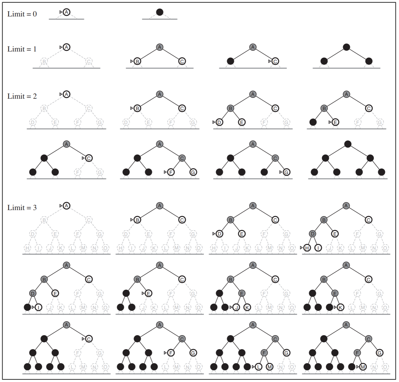
- Properties of Iterative Deepening DFS:
- Optimality: Optimal, if all the edges have the same edge cost
- Complete: by iteratively increasing the limit, at some point the algorithm reaches the goal and the algorithm never searches an infinite path
- Time Complexity: \(O(b^d)\), the number of nodes using depth limit, d, is equal to the number of nodes using all depths that are < d.
- Space Complexity: \(O(b^d)\), which is also the same as BFS.
Bidirectional Search
- Runs two simultaneous BFS searches: one forward from the initial state, and one backward from the goal.
- Then stop when both of the two BFS searches meet.
- Bidirectional search properties:
- Complete: Complete, if the branching factor, b, is finite
- Optimality: Optimal, if all the edges have the same cost, similar to BFS
- Time complexity: \(O(2b^{(\frac{d}{2})}) = O(b^{(\frac{d}{2})})\)
- Space complexity: \(O(2b^{(\frac{d}{2})}) = O(b^{(\frac{d}{2})})\)
Summary of Uninformed Search Strategies
| Method | Complete? | Time complexity | Space Complexity | Optimal? |
|---|---|---|---|---|
| BFS | Yes - If b is finite | \(O(b^d)\) | \(O(b^d)\) | Only if all edge costs are equal |
| DFS | No | \(O(b^m)\) | \(O(b \cdot m)\) | No |
| Uniform Cost | Yes - If b is finite | \(O(b^{1 +\lfloor C^{*}/\epsilon \rfloor})\) | \(O(b^{1 +\lfloor C^{*}/\epsilon \rfloor})\) | Yes |
| Iterative Deepening DFS | Yes | \(O(b^d)\) | \(O(b \cdot d)\) | Only if all edge costs are equal |
| Bidirectional BFS | Yes | \(O(b^{(\frac{d}{2})})\) | \(O(b^{(\frac{d}{2})})\) | Only if all edge costs are equal |
Informed(Heuristic) Strategies
Best-First Search
- Best-first search is a generalized category of heuristic based search.
- Informed search strategies use problem-specific knowledge beyond the definition of the problem
- General Approach: Best-first search is identical to uniform-cost search except that it uses a general evaluation function \(f(n)\), instead of the cost function \(g(n)\), for choosing which node to expand.
- The evaluation function, \(f(n)\), often contains a component, h, known as the heuristic function.
-
\(h(n)\) is the estimated cost of the cheapest past from the state at node, n, to the goal state
-
Straight-Line Distance(SLD) Heuristic - Choose \(h(n)\), as the straight line distance from node, n, to the goal state
-
Manhattan Distance Heuristic - Choose \(h(n)\), as the distance based strictly on vertical and horizontal distance as opposed to the SLD heuristic. This is like measuring the distance from one point to another in the city of Manhattan, which is shaped like a grid.
-
Greedy Best-First search - \(f(n) = h(n)\). Consequently, the node that seems to be the closest to the goal is expanded first. So it chooses the node with the lowest heuristic first.
- An example of Greedy Best-First search is
- The algorithm for recursive Best-First search is
function RECURSIVE-BEST-FIRST-SEARCH(problem) returns a solution, or failure
  return RBFS(problem, MAKE-NODE(problem.INITIAL-STATE), inf)

function RBFS(problem, node, f_limit) returns a solution or failure and a new f-cost limit
  if problem.GOAL-TEST(node.STATE) then return SOLUTION(node)
  successors <- []
  for each action in problem.ACTIONS(node.STATE) do
    add CHILD-NODE(problem, node, action) into successors
  if successors is empty then return (failure, inf)
  for each s in successors do // update f with value from previous search, if any
    s.f <- max(s.g + s.h, node.f)
  loop do
    best <- the lowest f-value node in successors
    if best.f > f_limit then return (failure, best.f)
    alternative <- the second-lowest f-value among successors
    result, best.f <- RBFS(problem, best, min(f_limit, alternative))
    if result != failure then return result
- Properties of Greedy-Best First search are
- Complete: Not complete, because it can get stuck if it does not keep track of the visited states. It can be complete if we keep track of the visited state
- Time Complexity: \(O(b^m)\), where m is the length of the longest path along the tree. Greedy Best First search can potentially search the entire tree.
- Space Complexity: \(O(b^m)\), we have to remember the whole tree to avoid redundant paths
A* search
- A* search is the most popular search algorithm
- It is similar to Greedy-Best First search, but it also takes the distance already traveled into account.
- The evaluation function, f, is defined as \(f(n) = g(n) + h(n)\)
- \(g(n)\) - the path cost from the start node to the node n
- \(h(n)\) - the estimated cost of the cheapest path from n to the goal
- \(f(n)\) - the estimated cost of the cheapest solution through n
- Admissibility of heuristics
- A heuristic function is admissible if it never overestimates the cost to reach the goal
- \(\forall n: h(n) <= h*(n)\), where \(h*(n)\), is the true cost of the shortest path from node n to the goal.
- By nature, admissible heuristics are also optimistic. An example of an admissible heuristic is SLD, because the straight line is the shortest distance between any two points, so it cannot overestimate the distance.
- Consistency or Monotonicity of heuristics
- A heuristic can be consistent if, for every node, n, and every successor, n’, of n generated by any action, a, the estimated cost of reaching the goal from n is no greater than the step cost of getting to n’ plus the estimated cost of reaching the goal from n’:
- Optimality of A*
- A* using tree search is optimal if the heuristic is admissible.
- A* using graph search is optimal if the heuristic is consistent.
- The proof of the optimality of A* follows directly from the following lemma:
Assume h is admissible.
Let n be a node such that n.State = goal and n is not the optimal path to the goal.
Let n' be the first node on the optimal path that is not on the path to n.
Then A* expands n' before n.
-
This means that A* will always expand all the nodes on the optimal path before expanding any non-optimal node that contains the goal. Therefore, A* is optimal.
- To prove the lemma above:
- Let’s denote the cost of the optimal path by C, \(C*(n) = g(n) + h*(n)\), C is also know as h* of the root node.
- When a non-optimal node n(that has n.STATE = goal) is created and added to the open-list, we compute its value \(f(n)\).
- Since n.STATE = goal, then \(f(n) = g(n)\)(real cost from root to n).
- The first optimal node n’ that has not yet been expanded has a value of \(f(n') = g(n') + h(n') <= C* <= g(n) = f(n)\)
- The first inequality follows from the admissibility of h and the second one follows from the definition of the minimum cost.
- Therefore, n’ should be expanded before n.
- For graph search A*, we need a stronger requirement on h because repeated states are not allowed
- A heuristic function, h, is said to be consistent if \(\forall (n, a, n'): h(n) <= c(n, a, n') + h(n')\), where \(c(n, a, n')\) is the step cost for going from n to n’ using action a.
- If h is consistent, then the graph search A* is optimal.
Designing Heuristics
- For many problems the procedure to generate a good heuristic is not trivial.
- Considering the 8-puzzle problem:
- One idea for a heuristic is the number of tiles that have to be moved so that the current state looks like the goal state
- Another idea for a heuristic is the sum of the Manhattan distances for all tiles between the current state and the goal state
- In A* search, we prefer heuristics that will allow us to expand as few nodes as possible.
- One way to evaluate the number of nodes expanded by a search technique is the effective branching factor b, and is defined as \(N = 1 + b^* + ( b^* )^2 + ... + ( b^* )^d\), where N is the number of nodes generated by A.
- The optimum and desired performance is for the effective branching factor to be 1.
Combining Heuristics
-
There are several times where we have several heuristics and there is not one heuristic that dominates the others. In this case, we could combine several heuristics.
-
If we have heuristics of \(h_1 , h_2 , h_3 , ... , h_n\), then we can calculate a new heuristic \(h_(max) = max { h_1 , h_2 , ... , h_n }\).
- It then follows that if the individual heuristics are admissible then the \(h_max\) is also admissible, because it can still never overestimate the actual, most optimal path, to get to the goal. Also if the individual heuristics are consistent, then \(h_max\) is also consistent.
Local Search
- Local search is suitable for optimization problems, where we plan to find the best state according to a given objective function.
- Local search have two advantages:
- They use little memory as they usually don’t need to remember paths
- They can often find reasonable solutions in large (or infinite) state spaces where systematic search is unsuitable.
Hill-climbing search (Greedy-local search)
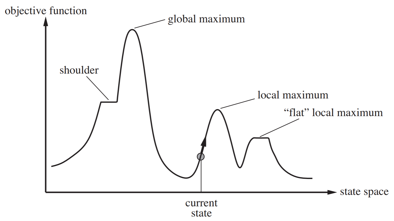
- Hill-climbing search is just looking at the left and right neighbors of the current position on a “hill”, then moving towards the higher valued neighbor compared to the current position.
- This image summarizes hill-climbing search and shows the difference between a local maximum and global maximum
- An algorithm for hill-climbing search is
function HILL-CLIMBING(problem) returns a state that is a local max
  current <- MAKE-NODE(problem.INITIAL-STATE)
  loop:
    neighbor <- highest-valued successor of current
    if neighbor.VALUE <= current.VALUE then return current.STATE
    current <- neighbor
- Scenarios where hill-climbing search has trouble:
- It gets stuck at plateaus or “flat” local maximums
- It also get stuck at ridges. Ridges are a sequence of local maxima that don’t directly connect to each other
- How to avoid shoulders?
- Starting from a random initial 8-queens state, hill-climbing gets stuck in a local maximum 86% of the time (with an average of 3 steps) and finds the global maximum only 14% (with an average of 4 steps)
- Sideways moves
- To avoid staying stuck in a shoulder plateau, wee allow hill-climbing to move to neighbor states that have the same value of the current one.
- However, infinite loops may occur. We can avoid the infinite loops by limiting the number of sideways moves.
- By allowing up to 100 sideways moves in 8-queens problem:
- We increase the percentage of problem instances solved by hill-climbing from 14% to 94%
- However, each successful instance is solved in 21 steps (on average) and failures (local maxima) are reached after 64 steps (on average)
Variants of hill-climbing
- Stochastic hill-climbing
- Chooses randomly among the uphill moves, with probabilities that vary with the steepness of the moves
- Converges slowly, but explores the state space better, and may find better solutions
- First-choice hill-climbing
- Generates successors randomly until finding one that is better than the current state.
- Efficient in high dimensions
- Random-restart hill-climbing
- Repeats the hill-climbing from a randomly generated initial state, until a solution is found.
- Guaranteed to eventually find a solution if the state space is finite.
- The expected number of restarts is \(\frac{1}{p}\) if hill-climbing succeeds with probability p at each iteration
Simulated Annealing
- Simulated Annealing is a widely used method for solving combinatorial optimization problems, such as VLSI, factory scheduling, and structural optimization
- Motivated by an analogy of annealing in solids:
- Heat the metal to a high temperature to increase the size of the crystals and reduce the defects. Then cool it down slowly, until the particles arrange themselves in the ground state of the solid. The ground state of the solid is a state of minimum energy of the solid.
- Steps for simulated annealing:
- Initialize the search with a random chosen state, and set the temperature T to a high value.
- Move in a random direction for a fixed distance.
- Calculate the value of the objective function in the new state and compare it to the value in the old state.
- If the value has increased, then stay in the new state. If the value has decreased, stay in the new state with a probability that is proportional to the change in value, otherwise move back to the old state.
- Decrease the temperature and return to Step 2.
- A simulated annealing algorithm:
function SIMULATED-ANNEALING(problem, schedule) returns a solution state
  inputs: problem <- a problem
          schedule <- a mapping from time to "temperature"

  current <- MAKE-NODE(problem.INITIAL-STATE)
  for t=1 to inf do:
    T <- schedule(t)
    if T=0 then return current
    next <- a randomly selected successor of current
    delta_E <- next.VALUE - current.VALUE
    if delta_E > 0 then current <- next
    else current <- next only with probability exp(delta_E/T)
Local Beam Search
- Local beam search is similar to running hill-climbing k times.
- In a local beam search, the k search paths are not independent. The successors of the k states are compared with each other.
-
States with many good successors dominate local beam searches.
- Steps for local beam search:
- Start with k randomly chosen initial states
- At each step, generate all the successors of the k states, and retain the k best ones
- Stop when a goal state is reached or when no further local improvement is possible
- Local beam search suffers from a lack of diversity among k paths. The search often ends up in a concentrated small region.
- Stochastic local beam search overcomes this problem by randomly generating the successors and keeping them with probabilities proportional to their values.
Genetic Algorithms
- Similar to local beam search, except that successors are generated by combining two parent states.
- Inspired from biological evolution through natural selection.
- A population is a set of individuals, each individual is a state represented as a string over a finite alphabet.
- A fitness function is used to select individuals that will reproduce.
-
Fitness function is a term used in genetic algorithms to describe objective functions.
- Example with the 8 queens problem:
- State: the positions of the 8 queens, each in a column of 8 squares. Each state is described by a sequence of \(8 \cdot \log_2 8 = 24 bits\)
- Fitness: number of pairs of queens that are not attacking each other(maximum = 28)
- A genetic algorithm consists of the following steps:
- Selection: Randomly drawing k individuals from the population with probabilities from the population with probabilities to their fitness. The same individual can be selected multiple times.
- Crossover: Let \((s_1 , s_2)\) be a selected couple of individuals, and let n be the size of the alphabet, and set s[i] be the i-th letter in the code of state s.
- Uniformly sample a random number \(i \in [1,n].]\)
- Create a new individual \({s'}_{1}\) that has the code \([{s'}_{1}[1], {s'}_{1}[2], ..., {s'}_{1}[i], {s'}_{2}[i+1], {s'}_{2}[i+2], ..., {s'}_{2}[n]]\)
- Create a new individual \({s'}_{2}\) that has the code \([{s'}_{2}[1], {s'}_{2}[2], ..., {s'}_{2}[i], {s'}_{1}[i+1], {s'}_{1}[i+2], ..., {s'}_{1}[n]]\)
- Mutation: Each letter in the codes of the new individuals is changed to a random value with a very small probability \(\eta\).
Optimization in continuous spaces
- Suppose that we want to construct three new airports in a given country.
- Objective: Minimize the distance from each city to its nearest airport.
- Solution:
- Let \(C_i\) denote the cities that have airport i as their nearest airport. Let \((x_i, y_i)\) be the coordinates of airport i and \((x_c, y_c)\) be the coordinates of city c. The objective is to optimize the function:
Gradient Descent
- A common approach for solving optimization problems consits in computing the gradient of the objective function f, and applying the update rule, \(x <- x - \alpha \nabla f\)
$$ \nabla f = (\frac{\partial f}{\partial x_1}, \frac{\partial f}{\partial y_1}, \frac{\partial f}{\partial x_2}, \frac{\partial f}{\partial y_2}, \frac{\partial f}{\partial x_3}, \frac{\partial f}{\partial y_3})
Adversarial Search
- Games
- Multiagent environments are environments where more than one agent is acting, simultaneously or at different times.
- Contingency plans are necessary to account for the unpredictability of the other agents.
- Each agent has its own personal utility function.
- The corresponding decision-making problem is called a game.
- A game is competitive if the utilities of different agents are maximized in different states.
- In zero-sum games, the sum of the utilities of all agents is constant.
- Zero-sum games are purely competitive.
- A game is described by:
- \(S_0\) - the initial state (How is the game setup at the start?)
- Players(s) - Indicates which player has the move in state s (Who’s turn is it?)
- Actions(s) - Set of legal actions in state s
- Result(s, a) - Returns the next state after we play action a in state s
- Terminal-Test(s) - Indicates if s is a terminal state
- Utility(s, p) - (also called objective or payoff function) - defines a numerical value for a game that ends in terminal state s for player p
Minimax algorithm
- Suppose that there are two players in a zero sum game:
- We call our player MAX, she tries to maximize our utility.
- We call our opponent MIN, she tries to minimize our utility
- Algorithm for Minimax
function MINIMAX-DECISION(state) returns an action
  return argmax(a in ACTIONS(s))(MIN-VALUE(RESULT(state, a)))

function MAX-VALUE(state) returns a utility value
  if TERMINAL-TEST(state) then return UTILITY(state)
  v <- -inf
  for each a in ACTIONS(state) do
    v <- MAX(v, MIN-VALUE(RESULT(s, a)))
  return v

function MIN-VALUE(state) returns a utility value
  if TERMINAL-TEST(state) then return UTILITY(state)
  v <- inf
  for each a in ACTIONS(state) do
    v <- MIN(v, MAX-VALUE(RESULT(s, a)))
  return v
- Some issues with Minimax:
- What if our opponent is not optimal? Can we still learn the opponent’s behavior?
- What if our player is trying to fool us by behaving in a different way?
- Aka hustling our player
- Minimax strategy in multiplayer games
- We have 3 players: A, B, and C
- The utilities are represented by a 3-dimensional vector: \((v_A, v_B, v_c)\)
- We apply the same principle; assume that every player is optimal
- If the game is not zero-sum, implicit collaborations may occur.
Alpha-Beta Pruning
- Time is a major issue in game search trees. Searching the complete tree takes \(O(b^m)\) operations, where b is the branching factor and m is the depth of the tree.
- Do we really need to parse the whole tree to find a minimax strategy? Is there any way to reduce the number of operations?
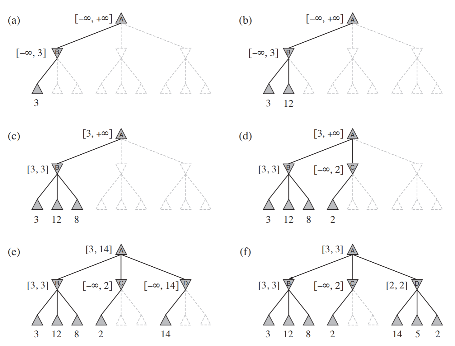
-
When we go through a game search tree, we can remove the other neighbor branches if we get a yield lower than or equal to the first highest yield found.
- Example of alpha-beta pruning:
Imperfect fast predictions
- The minimax algorithm generates the entire search tree
- The alpha-beta pruning algorithm allows us to prune large parts of the search tree, but its complexity is still exponential in the branching factor (number of actions).
-
This is still non-practical because moves should be decided quickly.
- Cutting off the search
- A cutoff test is used to decide when to stop looking further in the tree
- A heuristic evaluation function is used to estimate the utility where the search is cutoff
- Evaluation functions must be computed very quickly